Traditional Vs Neural Networks

A traditional approach while programming is when a programmer manually specifies the rules that the program should use. For example, in the case of identifying a cat or dog from an image, the programmer might write code to look for certain features, such as pointy ears or a long tail, and use these features to classify the given image as a cat or a dog.

But neural networks are a type of machine learning algorithm that can learn on their own from examples shown to it without being explicitly programmed with any rules.

So in the above example of classifying an image as a dog or cat, a Neural network is trained on a dataset of many such as images of cats and dogs, and it learns to eventually classify any new image as a cat or dog on its own.

This makes neural networks more flexible and adaptable to new tasks, as they can learn to recognize patterns and features that may not be apparent to a human programmer’s assumptions.

Artificial Neural Networks (ANN)

Artificial neural networks (ANNs) are computational models inspired by the structure and function of the human brain. They are composed of many interconnected processing nodes, known as neurons, that work together to solve complex problems. One of the key algorithms used in training ANNs is Gradient Descent (GD), which is used to minimize the error or cost function of the network. In this blog, we will discuss the basics of ANNs and GD and how they work together to create powerful machine-learning models.

What is a Neuron

Let us start with understanding what is a neuron .

A neuron is the basic unit of an ANN, which receives input signals from other neurons or external inputs, processes them, and generates an output signal.

A neuron is represented as a simple function that takes one or more inputs and produces an output based on its internal parameters or weights. The connection between neurons is represented by synapses, which are weighted connections that determine the strength of the connection between neurons.

Let’s take an example of a network that has a single neuron to understand the concept better.

The below picture represents a single neuron is the simplest representation of an Artificial neural network and is presented here for ease of understanding.

Figure 1

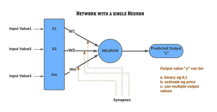
Here the neuron takes Input values similar to our senses (X1 to Xm) and the output (y) is an output value generated after processing the information in the neural network.

Note: output value “y ” can be:

1. continuous (eg salary or price of something ) like regression
2. Classification or probability (probability of something happening) as in logistic regression.
3. Or it can even have several output variables where each of the output values can utilize 1. or 2.

The connection between the neurons is called the synapse and each synapse is assigned a weight (W1 to W3).

Let’s take another example to understand the concept of a neuron better. Consider a scenario where we want to predict the salary of an individual based on factors like age, years of experience, and educational background.

We can represent this as an input-output mapping problem, where the input values are the independent variables (age, years of experience, educational background, etc.), and the output value is the dependent variable (salary).

In the above example, the Input values are independent variables and are age, the number of years of experience, educational background, etc, and the Output value is the salary of the person.

Training an Artificial Network

As we have seen in Figure 1, the synapses connecting the input values to the neuron have weights. During the training process, these weights are adjusted.

Initially, these weights are all initialized to random values and during the training process they are fine-tuned while minimizing the error or cost function.

But how that’s done?

Let’s say we want to train a neural network to predict salaries based on age, years of experience, and educational background.

After the network has been trained, we could use it to predict the salary of a new person based on their age, years of experience, and educational background.

The Training Dataset

The first thing we would need is a training dataset that provides the actual salaries of people with varying ages, years of experience, and educational backgrounds.

But the training dataset would need to be large enough to provide sufficient examples for the network to learn from, and it should also be diverse enough to capture a wide range of salaries based on the input features.

We should have a data set like the below example but in a real scenario it should have many more rows

Figure 2

Here each row represents ages, years of experience, educational backgrounds, and actual salary of an individual represented above as “y”.

Calculating the Predicted Output value and the Cost Function

Let’s refer again to Figure 1,

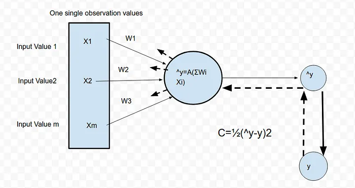
We can see the weights represented as W1, W2, W3 are associated with each synapse. During training, these weights are fine-tuned while minimizing the cost function (C) which we have chosen.

To start with we sum up the weights and input values below to come up with an output value which is a predicted value represented by ŷ.

In Figure 1, which uses a single neuron our input values are X1, X2, and Xm, and they are connected to a neuron using weights W1, W2, and W3

So inside the neuron, we sum up like below to get an output value

ŷ = X1*W1+X2*W2+………Xm*W3

This can also be represented mathematically as

ŷ= Σ WiXi (Where i=0 to m)

Here,

Wi = is the weight value of each synapse

Xi =is the input value connected to each synapse

ŷ = is the predicted value that the network is outputting currently

y= is the actual value that we have used in the training dataset

The value ŷ and y is now used to calculate a cost function

Cost function

In machine learning, a cost function, also known as a loss function, is a mathematical function that measures the difference between the predicted output of a machine learning model and the actual output from the training dataset. The goal of the cost function is to provide a measure of how well the model is performing and to guide the learning process by minimizing its value.

For simplicity, Let’s use a mean squared cost function. Note how both ŷ and y are used to calculate the cost function.

An MSE cost function can be represented as

C = 1/2m Σ ( ŷ -y)2

Note: For some networks, there can be only weights but some networks have both weights and biases. For simplicity on how a network works, the above-explained weights.

Some additional reading can be done here on the role of biases in the below link

Epoch

In neural network training, an epoch refers to a single pass through the entire training dataset during the training process. During an epoch, the neural network is trained on all of the available training data, typically using a batch-based approach where the data is split into smaller batches and each batch is used to update the network’s weights and biases.

In practice, it is common to train a neural network for multiple epochs, where each epoch involves a complete pass through the training data. This helps to improve the performance of the network by allowing it to learn from the data over multiple iterations. The number of epochs used during training is a hyperparameter that can be tuned to optimize the performance of the network.

Forward and Backpropagation

The input data or information is passed forward through the neural network and the output is computed. That is with each set of input values (x1..xm) and we get y^ (ie the predicted value ). Which is then used to check with the actual value y using a cost function. This is called forward propagation.

After the error or loss is computed by comparing the predicted output with the actual output. The error is then propagated backward through the network to update the weights and biases of the network using the gradient descent algorithm(Which is explained in more details below.) .This is called Back Propagation.

The goal of backpropagation is to reduce the cost function during training.

Backpropagation is actually a very advanced algorithm that adjusts the weights all at the same time.

If you want to know more about these algorithms, then please check out.

http://neuralnetworksanddeeplearning.com/chap2.html

Normalization

Before training the input values should be standardized /normalized so that they are very similar to each other.

Normalization is an important preprocessing step in artificial neural networks (ANNs) that involves scaling the input values so that they have similar ranges and distributions.

When the input values are not normalized, it can cause problems during the training process. For example, if some input features have large values compared to other features, the network may assign more importance to the larger features during training. This can cause the weights and biases of the network to become imbalanced, which can lead to poor performance on new data.

By normalizing the input values, we can ensure that each feature is given equal importance during training, which can improve the performance of the network.

For more information on normalization, refer to the below paper which is by Yann Lecun who is also the founding father of convolutional nets,

http://yann.lecun.com/exdb/publis/pdf/lecun-98b.pdf

The Training Algorithm

The basic idea behind training is that we try to reduce the cost function by adjusting the weights and biases.

Say we have a data set for example where we want to predict the salary of a person based on age, education, and the number of years of experience and we use the network below to find the salary or output value.In which we use the mean squared cost function.

Here is what happens during the training

• We start with random weights
• We input each row into the network we get an output value ŷ as the predicted value.
• we use a cost function also known as the loss function to compare the predicted value(ŷ) with the actual value (y). we used a Mean Square Cost function in the diagram below
• This information is then backpropagated in the network to adjust the weights as shown in the diagram below.
• The goal is to minimize the cost function and to make the cost function zero by adjusting the weights with each iteration.

In the real world, we train the network with millions of data sets, and eventually, the weights are optimized so that the cost function or the loss function is minimum

So, the whole training process can be represented as the diagram below

Figure 3:

Activation function

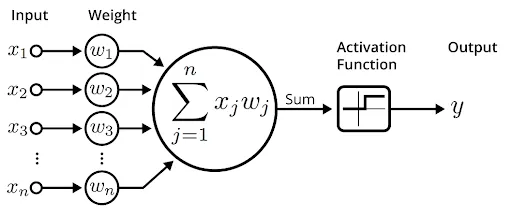
An activation function is a mathematical function that is applied to the output of each neuron in a neural network to determine whether the neuron should be activated or not.

The activation function serves as a threshold for determining whether the output of the neuron should be considered significant or not. If the output of the neuron is above the threshold set by the activation function, the neuron is activated and its output is passed on to the next layer of the network. If the output is below the threshold, the neuron is not activated and its output is not passed on

So finally a working ANN network will look like below

Figure 4

There are several popular activation functions used in neural networks,

The most popular among them are the sigmoid function and the rectified linear unit (ReLU) function as described below.

But there are other activation functions including the hyperbolic tangent (tanh) function. Each activation function has its own advantages and disadvantages, and the choice of activation function can have a significant impact on the performance of the network.

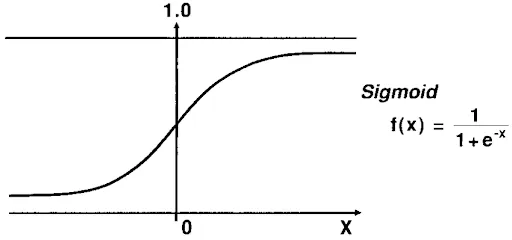
A sigmoid function

The sigmoid function is a smooth, S-shaped curve that maps the output of the neuron to a value between 0 and 1, Sigmoid never becomes 1 or 0, and particularly this activation function is used for prediction and probability of something to occur.

The mathematical formula for a sigmoid function is represented below

Where x is the input value and where e ≈ 2.71 is Euler’s Number and is the base of the natural logarithm

Rectifier function

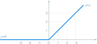
The ReLU function, on the other hand, is a simple piecewise linear function that maps all negative inputs to 0 and all positive inputs to their own value.

Rectifier function is mostly used in Convolutional neural networks for computer visions application.

It can be represented mathematically as

f(x)=max (x,0)

ie if the value is less than 0, then the output is 0, or else the value itself

It can produce a graph like below

Figure 6

More advanced Neural network with Hidden Layers

While a single neuron can be useful in some cases, neural networks typically consist of multiple layers of neurons.

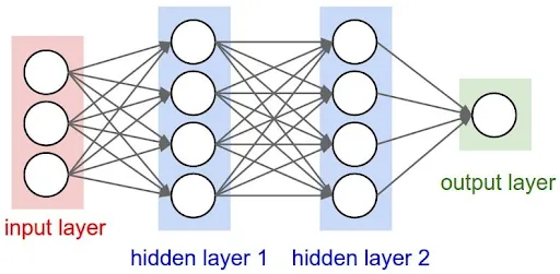
A neural network typically consists of an input layer, one or more hidden layers, and an output layer. The input layer receives the input data, which is then passed through the hidden layers to generate the output. Each layer of neurons is connected to the next layer through a set of weights and biases.

The design of a neural network involves choosing the appropriate number of layers, neurons, and activation functions, as well as selecting an appropriate optimization algorithm and loss function to minimize the error of the network.

A Typical neural network may look like below

Figure 7

Some important points to note here are.

1. Some of the weights can have a 0 value this is because some neurons may not be interested in some of the input values.

Take Example 2, where we wanted to predict the salary of a person based on age, years of experience, and so on, and say that for some scenarios the age of the person does not determine the salary, in that case, the synapses connecting the Age input value to a neuron will be Zero

Gradient Descent

Let’s see now how the cost is reduced and how the cost function is minimized by adjusting the weights. But first, we should understand that, If we use the brute force method( ie try out all the weights possible randomly) then it will take forever to train a network even for a supercomputer.

To make it easier, one of the mathematical terms used to adjust the weights is called gradient descent which we hear often.

So, Let’s try to understand Gradient Descent and how it helps to optimize the weights

Refer to the picture below (Figure 8), The basic idea behind gradient descent is to start at a random point (i.e., start with initial random weights and biases) and then we find what the slope is (from the initial point).

Once we do that we can apply the below logic

• If the slope is negative then go left.
• If the slope is possible then go right.

And just by understanding which way we need to adjust the weights by measuring the slope, we can arrive at a minimum.

For example, change some weight and see which way we are going with respect to cost function and correct yourself.

Figure 8

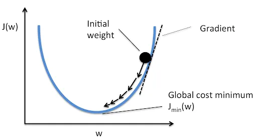
Gradient descent speeds things up training drastically. And by repeatedly applying the gradient descent algorithm over the training dataset, the weights and biases of the neural network are gradually adjusted to minimize the cost function

Stochastic gradient descent

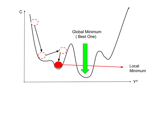
One of the biggest problems with Gradient Descent is that it needs the cost function to have one global minimum( ie the cost function has to be convex ). Or it can get stuck in local minima and not converge to global minima.

Local minima are points in the parameter space where the cost function has a lower value than its neighbors, but not necessarily the lowest value in the entire parameter space which is the global minima of the entire parameter space.

This happens when the training data is more erratic and random.

For example, in the diagram below we can end up in the red instead of the global minimum(green)

Figure 9

To overcome these problems, one of the methods used is stochastic gradient descent which is a variant of Gradient Decent.

Unlike batch gradient descent, which updates the weights and biases of the network after processing the entire training dataset, SGD updates the weights and biases after processing a single training example or a small batch of training examples.

This avoids local minimum as it has much higher fluctuations and is much more likely to find a global minimum instead of a local minimum. Moreover, it makes the training much faster.

But note:

• Gradient descent is more deterministic in its results

The important thing to note here is that Gradient Descent and Stochastic Gradient descent are methods used for training and adjusting the weights to get an optimal ŷ and minimum cost.

If you are interested in knowing more about the mathematical theory of gradient descent and stochastic gradient descent. Please check out the blog below

https://iamtrask.github.io/2015/07/27/python-network-part2/?source=post_page—–2ebda025c6f9—————————————